machine learning – Notes of a Neuropsychiatry Amateur

RNN-based encoder – decoder architecture explained

RNN-based Encoder – Decoder

Encoder
An encoder transforms the input data into a different representation, usually a fixed-size context vector. The input data x can be a sequence or a set of features. The encoder maps this input to a context vector c, which is a condensed representation of the input data. Mathematically, this can be represented as:

$\textbf{c = f(x)}$
$c \text{ - context vector, } x \text{ - input data}$

In the case of a sequence, such as a sentence in a language translation task, the encoder might process each element of the sequence (e.g., each word) sequentially. If the encoder is a recurrent neural network (RNN), the transformation f can involve updating the hidden state h at each step:

$\boldsymbol{h_t = f(h_{t-1}, x_t)}$
$h_t \text{ - hidden state at time } t$
$x_t \text{ - input at time } t$
$h_{t-1} \text{ - hidden state at time } t-1$

The final hidden state h_T can be used as the context vector c for the entire input sequence.

Decoder
The decoder takes the context vector c and generates the output data y. In many applications, the output is also a sequence, and the decoder generates it one element at a time. Mathematically, the decoder’s operation can be represented as:

$\boldsymbol{y_t = g(y_{t-1}, h_t, c)}$
$y_t \text{ - output at time } t$
$h_t \text{ - hidden state at time } t$

In many sequence-to-sequence models, the decoder is also an RNN, and its hidden state is updated at each step:

$\boldsymbol{h_t = g(h_{t-1}, y_{t-1}, c)}$

The encoder-decoder framework, particularly in the context of sequence-to-sequence models, is designed to handle sequences of variable lengths both on the input and the output sides.

Output Generation (Decoder)

Initial State: The decoder is initialized with the context vector c as its initial state:

$h'_0 = C$

Start Token: The decoder receives a start-of-sequence token SOS as its first input y0.
Decoding Loop: At each step t, the decoder generated an output token y_t and updates its hidden state h’_t.
Variable Length Output: The decoder continues to generate tokens one at a time until it produces an end-of-sequence token EOS. The length of the output sequence Y = (y_1, y_2, …, y_m) is not fixed and can be different from the input length n. The process is as follows:

$y_t = Decode(h'_{t-1}, y_{t-1})$
$h'_t = UpdateState(h'_{t-1}, y_{t-1})$
$\text{for t = 1 to m, where m can be different from n}$

Stopping Criterion: The loop stops when the EOS token is generated, or after producing the maximum allowed length for the output sequence.

The decoder can be also represented using the probability distribution of the next token given the previous tokens and the context vector c from the encoder:

$p(y_t|y_{<t}, C)$

The full sequence probability is the product of individual token probabilities: the decoder generates a sequence token by token, and the probability of the sequence Y given the context vector C can be described by the chain rule of probability:

$p(Y|C) = p(y_1|C) * p(y_2|y_1, C) * ... * p(y_m|y_{<m}, C)$

How do we obtain these conditional probabilities?
– For each time step t from 1 to m (m is to be determined):

$\bullet \text{The decoder takes the previous hidden state } h'_{t-1} \text{ and the previously generated token } y_{t-1}$
$\text{ as inputs.}$
$\bullet \text{The function } f_{theta_{dec}} \text{, parametrized by decoder's weights } \theta_{dec} \text{, computes the current}$
$\text{ hidden state } h'_t \text{ and the logit vector } l_t \text{, which precedes the probability distribution}$
$\text{for the next token.}$
$(h'_{t-1}, y_{t-1}) \xrightarrow{f_{\theta_{dec}}} (l_t, h'_t)$
$\bullet \text{The logit vector is computed by multiplying the embedded representation of the decoder's}$
$\text{output by the transposed word embedding matrix}$
$l_t = W_ey' + b$
$\bullet \text{The logit vector } l_t \text{ is passed through a softmax layer to obtain the probability}$
$\text{distribution for the next token } y_t:$
$p(y_t | y_{<t}, C) = Softmax(l_t)$

Token Generation:

$\bullet \text{A token is sampled from the probability distribution } p(y_t|y_{<t}, C) \text{, which becomes}$
$\text{the next token in the sequence } y_t$
$\bullet \text{This token is then used as the input for the next time step}$

Sequence Continuation:
– This process repeats, with the decoder generating one token at a time, updating its hidden state, and adjusting the probability distributions for subsequent tokens based on the current sequence.

Stopping Criterion:
– The loop continues until the decoder generates an EOS token, indicating the end of the sequence, or until it reaches a predefined maximum sequence length.

Using Objective/Technical Reading as a Tool Against Depressive Rumination

I have been diagnosed with clinical depression since 2015, it’s been on and off. Because of this diagnosis, I naturally became interested in medical and talk therapy treatments for depression. In grad school, I had the opportunity to work with a dataset of Facebook posts of users who also had labels as depressed and non-depressed, based on the standard clinical questionnaire.

Using natural language processing (NLP) techniques, one of my findings was that depressed people use more personal pronouns in their text, such as “I”, “he”, “she”, and “we”. For instance, I noticed in my own experiences that when I am more depressed, I tend to ruminate more—thinking about how “I” am unlucky not to have many relatives, or how it’s unfair that he/she (some person that I know) is smarter or has a better job or a better life.

I found a skill that helps manage these thoughts. When I catch myself ruminating, I try to engage in reading something technical or objective that doesn’t involve personal pronouns or comparisons or human relationships in general. For example, I might read an article about Python vs Julia, or why high blood sugar is dangerous, or where turtles go in winter in Ontario. I find that even if the ruminative thoughts continue, forcing myself to read and focus on these kinds of articles can help prevent my ruminative thoughts from escalating.

I am not sure what type of skills this could be called – CBT or DBT, but I think it relates more to the DBT skill of “opposite action”. This skills is based on doing the opposite of what our emotions/mind is telling us to do. So if my mind is telling me to sit and ruminate about my life, myself, myself vs. others, I do the opposite – read something that doesn’t involve any personal life at all.

Percentile Confidence Interval Calculator

Percentile-Confidence-Interval-Calculation.ipynb

This Python script calculates the 95% confidence interval for a specified percentile (e.g., the 70th percentile) of a dataset. The confidence interval provides a range in which we expect the true percentile value to lie with 95% confidence.

The calculation makes use of the binomial distribution properties, making an assumption that our data can be modeled by a binomial distribution. This assumption may not always be accurate, especially for continuous data, but it provides an approximation for our purposes.

Assumptions

1. Binary Outcome: The fundamental assumption behind the binomial distribution is that there is a binary outcome, often termed as ‘success’ and ‘failure’. In the context of percentiles, you can think of ‘success’ as the instances below the percentile and ‘failure’ as the instances above.

2. Fixed Number of Trials: For the binomial distribution, there is a fixed number n of trials. In our case, n represents the total number of data points in our sample.

3. Independence: Each trial (or data point) is independent of others. This means the outcome of one trial does not affect the outcome of another.

4. Constant Probability of Success: The probability of success, q, is the same for each trial. Here, q represents the percentile value. For example, for the 70th percentile, q=0.7.

Why the Binomial Distribution?

The rationale behind using the binomial distribution for percentile confidence intervals is its direct applicability to cases where you’re looking at the proportion of observations below a certain threshold (i.e., a percentile).

When you’re asking about the 70th percentile, you’re essentially inquiring: “What’s the value below which 70% of my data falls?” This can be likened to asking about the number of successes in n trials, where a success is an observation below the desired threshold.

However, it’s important to note that this method provides an approximation. The binomial distribution is discrete and inherently based on counting successes in a set number of trials, while percentiles often come from continuous distributions and may not perfectly adhere to the assumptions above.

import numpy as np
from scipy.stats import binom
import seaborn as sns

Get some data

# Load the Iris dataset
iris = sns.load_dataset("iris")
# Use the 'sepal_length' feature
data = iris['sepal_length'].values

print(data[:50])

[5.1 4.9 4.7 4.6 5.  5.4 4.6 5.  4.4 4.9 5.4 4.8 4.8 4.3 5.8 5.7 5.4 5.1
 5.7 5.1 5.4 5.1 4.6 5.1 4.8 5.  5.  5.2 5.2 4.7 4.8 5.4 5.2 5.5 4.9 5.
 5.5 4.9 4.4 5.1 5.  4.5 4.4 5.  5.1 4.8 5.1 4.6 5.3 5. ]

Calculate the 70th percentile

# Calculate the 70th percentile
percentile_70 = np.percentile(data, 70)
print("Min: %f, Max: %f, 70th percentile: %f" % (min(data), max(data), percentile_70))

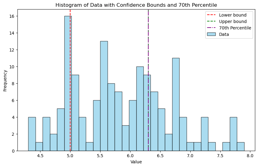
Min: 4.300000, Max: 7.900000, 70th percentile: 6.300000

Convert the data to “success” (above the 70th percentile) and “failure”

successes = np.sum(data > percentile_70)
failures = len(data) - successes

# Now, `successes` is analogous to `q * n` in the binomial scenario.
# So, we can set:
n = len(data)
q = successes / n

print("n: %d, q: %f" % (n, q))

n: 150, q: 0.280000

Calculate the 95% confidence interval

The code calculates potential upper (u) and lower (l) bounds for a confidence interval using the binomial distribution’s percent-point function (ppf).

np.ceil(binom.ppf(1 – alpha / 2, n, q)) determines the approximate upper bound for the confidence interval and np.ceil(binom.ppf(alpha / 2, n, q)) for the lower bound.

+ np.arange(-2, 3) extends these bounds by adding an array of [-2, -1, 0, 1, 2], generating a set of potential boundaries around the original estimate.

u gives a sequence of indices in the dataset that demarcate the upper bound of the confidence interval. It starts from the calculated index for the 97.5th percentile and provides two more indices above and two below it.

l gives a sequence of indices in the dataset that demarcate the lower bound of the confidence interval. It starts from the calculated index for the 2.5th percentile and provides two more indices above and two below it.

alpha = 0.05
u = np.ceil(binom.ppf(1 - alpha / 2, n, q)) + np.arange(-2, 3)
u[u > n] = np.inf

l = np.ceil(binom.ppf(alpha / 2, n, q)) + np.arange(-2, 3)
l[l < 0] = -np.inf

print("u: " + ", ".join(map(str, u)))
print("l: " + ", ".join(map(str, l)))

u: 51.0, 52.0, 53.0, 54.0, 55.0
l: 29.0, 30.0, 31.0, 32.0, 33.0

sorted_data = np.sort(data)

# Extract values corresponding to the indices
# Correct way to interpret the u and l values
u_values = sorted_data[n - u.astype(int)]
l_values = sorted_data[l.astype(int) - 1]

print("Upper values:", u_values)
print("Lower values:", l_values)

Upper values: [6.3 6.2 6.2 6.2 6.2]
Lower values: [5.  5.  5.  5.  5.1]

Probability coverage

The code calculates the probability coverage of different combinations of potential confidence intervals formed by the lower bounds (l) and upper bounds (u). Coverage is a matrix of probabilities. The goal is to find the smallest confidence interval that guarantees coverage of at least 1−α.

coverage = np.zeros((len(l), len(u)))
for i, a in enumerate(l):
    for j, b in enumerate(u):
        coverage[i, j] = binom.cdf(b - 1, n, q) - binom.cdf(a - 1, n, q)

if np.max(coverage) < 1 - alpha:
    i = np.where(coverage == np.max(coverage))
else:
    i = np.where(coverage == np.min(coverage[coverage >= 1 - alpha]))

print("Coverage Matrix:")
print(coverage)

print("\nOptimal Indices (i_l, i_u):")
print(i)

Coverage Matrix:
[[0.93135214 0.95028522 0.96430299 0.97438285 0.98142424]
 [0.92730647 0.94623955 0.96025732 0.97033718 0.97737857]
 [0.92096076 0.93989385 0.95391161 0.96399148 0.97103286]
 [0.91140808 0.93034117 0.94435894 0.9544388  0.96148018]
 [0.89759319 0.91652627 0.93054404 0.9406239  0.94766529]]

Optimal Indices (i_l, i_u):
(array([0], dtype=int64), array([1], dtype=int64))

i_l = i[0][0]
i_u = i[1][0]
print("Chosen row of coverage matrix: %d, chosen column of coverage matrix: %d" % (i_l, i_u))

u_final = min(n, u[i_u])
u_final = max(0, int(u_final)-1)
        
l_final = min(n, l[i_l])
l_final = max(0, int(l_final)-1)

# Actual value corresponding to u_final and l_final
upper_value_threshold = n - u_final
lower_value_threshold = l_final

upper_value = sorted_data[upper_value_threshold]
lower_value = sorted_data[lower_value_threshold]

print("Lower bound value:", lower_value)
print("Upper bound value:", upper_value)

Chosen row of coverage matrix: 0, chosen column of coverage matrix: 1
Lower bound value: 5.0
Upper bound value: 6.3

import matplotlib.pyplot as plt

# Plotting the histogram
plt.figure(figsize=(10, 6))
plt.hist(data, bins=30, color='skyblue', edgecolor='black', alpha=0.7, label='Data')

# Adding vertical lines for lower_value and upper_value
plt.axvline(lower_value, color='red', linestyle='--', label='Lower bound')
plt.axvline(upper_value, color='green', linestyle='--', label='Upper bound')

# Adding vertical line for the 70th percentile
plt.axvline(percentile_70, color='purple', linestyle='-.', label='70th Percentile')

# Adding title and labels
plt.title('Histogram of Data with Confidence Bounds and 70th Percentile')
plt.xlabel('Value')
plt.ylabel('Frequency')
plt.legend()

plt.show()

Bootstrap method

A commonly used alternative method to calculate confidence intervals for percentiles (also known as quantiles) is the Bootstrap method.

The Bootstrap method involves resampling the dataset multiple times with replacement and then computing the desired statistic (in this case, the 70th percentile) for each of these resampled datasets. This gives a distribution of the 70th percentiles from which we can compute the confidence interval.

lower: This represents the value below which the bottom 2.5% of your jotted down 70th percentiles fall. In other words, it’s like saying, “In 2.5% of our bootstrap ‘experiments,’ the 70th percentile was below this value.”

upper: This is the value below which the bottom 97.5% of your jotted down 70th percentiles fall. Put another way, “In 97.5% of our bootstrap ‘experiments,’ the 70th percentile was below this value.”

import numpy as np

def bootstrap_percentile_CI(data, percentile=70, alpha=0.05, B=10000):
    """Calculate the bootstrap confidence interval for a given percentile."""
    n = len(data)
    resampled_percentiles = []

    for _ in range(B):
        resample = np.random.choice(data, n, replace=True)
        resampled_percentiles.append(np.percentile(resample, percentile))

    lower = np.percentile(resampled_percentiles, 100 * alpha/2)
    upper = np.percentile(resampled_percentiles, 100 * (1-alpha/2))
    
    return lower, upper

# Calculate the bootstrap 70th percentile confidence interval
lower_bootstrap, upper_bootstrap = bootstrap_percentile_CI(data)
print("Bootstrap 70th percentile CI: (%.2f, %.2f)" % (lower_bootstrap, upper_bootstrap))

Bootstrap 70th percentile CI: (6.10, 6.43)

# Plotting
plt.hist(data, bins=30, color='lightblue', edgecolor='black', alpha=0.7)
plt.axvline(x=np.percentile(data, 70), color='green', linestyle='--', label="True 70th Percentile")
plt.axvline(x=lower_bootstrap, color='red', linestyle='--', label="Lower Bound of CI")
plt.axvline(x=upper_bootstrap, color='blue', linestyle='--', label="Upper Bound of CI")
plt.legend()
plt.title('Histogram of Sepal Length with Bootstrap CI for 70th Percentile')
plt.xlabel('Sepal Length')
plt.ylabel('Frequency')
plt.show()

Discussion

The bootstrap method makes minimal assumptions about the distribution of the data, making it versatile for a wide variety of datasets. This flexibility allows the bootstrap to handle complex or unknown data distributions, whereas the binomial method assumes data follows a binomial distribution and is mainly suited for binary outcomes. While the binomial approach is computationally simpler and quicker, it might not always provide an accurate representation, especially if the underlying assumptions aren’t met. In contrast, the bootstrap can be more computationally intensive due to resampling but offers the advantage of being more adaptable and often provides a more accurate estimate for datasets that don’t strictly adhere to a binomial distribution.

Fructose Malabsorption – Applying the Luhn algorithm for text summarization

The Luhn algorithm is a text summarization technique that uses statistical properties of the text to identify and extract the most important sentences from a document. The algorithm was developed by H.P. Luhn in the 1950s, and is still widely used in various forms today.

The Luhn algorithm works by first analyzing the frequency of each word in the document, and then assigning a score to each sentence based on the frequency of the words it contains. Sentences that contain words that are more frequent in the document as a whole are considered to be more important, and are assigned higher scores. The algorithm then selects the top-scoring sentences and concatenates them together to form the summary. The length of the summary is usually determined in advance by the user, and the algorithm selects the most important sentences that fit within that length limit.

It works by identifying the most salient or important sentences in a document based on the frequency of important words and their distribution within each sentence. First, the algorithm removes stopwords, which are common words such as “the”, “and”, and “a” that do not carry much meaning. Additionally, one could apply stemming, which reduces words to their base or root form. For example, “likes” and “liked” are reduced to “like”. Then, the algorithm looks for important words in each sentence. These are typically nouns, verbs, and adjectives that carry the most meaning. The specific method for identifying important words may vary depending on the implementation of the algorithm, but in general, they are selected based on their frequency and relevance to the topic of the text.

The algorithm counts the number of important words in each sentence and divides it by the span, or the distance between the first and last occurrence of an important word. This gives a measure of how densely the important words are distributed within the sentence. Finally, the algorithm ranks the sentences based on their scores, with the highest scoring sentences considered the most important and selected for the summary.

Here are the step-by-step instructions for the Luhn algorithm:

Preprocess the text: Remove any stop words, punctuation, and other non-textual elements from the document, and convert all the remaining words to lowercase.
Calculate the word frequency: Count the number of occurrences of each word in the document, and store this information in a frequency table.
For each sentence, calculate the score by:
a. Identifying the significant words (excluding stop words) that occur in the sentence.
b. Ordering the significant words by their position in the sentence.
c. Determining the distance between adjacent significant words (the “span”).
d. Calculating a score for the sentence as the sum of the square of the number of significant words divided by the span for each adjacent pair of significant words.
Select the top-scoring sentences: Sort the sentences in the document by their score, and select the top-scoring sentences up to a maximum length L. The length L is typically chosen by the user in advance, and represents the maximum number of words or sentences that the summary can contain.
Generate the summary: Concatenate the selected sentences together to form the summary.

Below I summarize the topic of fructose malabsorption by generating a summary using the Luhn algorithm. To create the summary, I selected several articles from sources like Wikipedia and PubMed. The important words were selected based on their total frequency in all of the text. I chose the top 25 words to focus on, and then used the algorithm to identify the most important sentences based on the frequency and distribution of these words. The summary was generated using the top 15 sentences.

Symptoms and signs of Fructose malabsorption may cause gastrointestinal symptoms such as abdominal pain, bloating, flatulence or diarrhea. Although often assumed to be an acceptable alternative to wheat, spelt flour is not suitable for people with fructose malabsorption, just as it is not appropriate for those with wheat allergies or celiac disease. However, fructose malabsorbers do not need to avoid gluten, as those with celiac disease must. Many fructose malabsorbers can eat breads made from rye and corn flour. This can cause some surprises and pitfalls for fructose malabsorbers. Foods (such as bread) marked “gluten-free” are usually suitable for fructose malabsorbers, though they need to be careful of gluten-free foods that contain dried fruit or high fructose corn syrup or fructose itself in sugar form. Food-labeling Producers of processed food in most or all countries, including the US, are not currently required by law to mark foods containing “fructose in excess of glucose”.

Stone fruit: apricot, nectarine, peach, plum (caution – these fruits contain sorbitol);Berry fruit: blackberry, boysenberry, cranberry, raspberry, strawberry, loganberry; Citrus fruit: kumquat, grapefruit, lemon, lime, mandarin, orange, tangelo; Other fruits: ripe banana, jackfruit, passion fruit, pineapple, rhubarb, tamarillo.

The fructose and glucose contents of foods listed on the Australian food standards would appear to indicate that most of the listed foods have higher fructose levels.

Glucose enhances absorption of fructose, so fructose from foods with fructose-to-glucose ratio <1, like white potatoes, are readily absorbed, whereas foods with fructose-to-glucose ratio >1, like apples and pears, are often problematic regardless of the total amount of fructose in the food.

Foods with high fructose-to-glucose ratio.

Dietary supplements of xylose isomerase may improve some symptoms of fructose malabsorption, although there is currently only a single scientific study available.

This can lead to issues such as bloating, heartburn and constipation.

It is called a hydrogen breath test and is the method currently used for a clinical diagnosis.

People with fructose malabsorption absorb less than 25 g per sitting.

Fructose malabsorption should be considered in patients with symptoms of depression and disturbances of tryptophan metabolism. This prospective cross-sectional study aimed to investigate the potential association between primary-adult lactose malabsorption, fructose malabsorption, tryptophan (TRP) metabolism and the presence of depressive signs.

High intestinal fructose concentration seems to interfere with L-tryptophan metabolism, and it may reduce availability of tryptophan for the biosynthesis of serotonin (5-hydroxytryptamine).

After obtaining the top sentences above, I used them as input into ChatGPT to generate another summary. The summary ended up with some mistakes, such as “People with this condition should avoid foods like spelt flour that contain fructose.“, as spelt does not contain fructose, it contains fructans. But it was still a fun exercise.

Fructose malabsorption can cause gastrointestinal symptoms such as abdominal pain, bloating, flatulence, and diarrhea. People with this condition should avoid foods like spelt flour that contain fructose. However, they do not need to avoid gluten, and many can eat breads made from rye and corn flour. Foods marked “gluten-free” are generally suitable for fructose malabsorbers, but they need to be careful of gluten-free foods that contain dried fruit or high fructose corn syrup. Certain fruits such as apricots, nectarines, peaches, and plums can cause issues due to their sorbitol content. The fructose-to-glucose ratio of foods can also play a role in absorption, with foods with a higher ratio often being problematic. A hydrogen breath test is used for clinical diagnosis, and dietary supplements of xylose isomerase may help with symptoms. Fructose malabsorption may also be associated with depressive signs due to the interference with L-tryptophan metabolism.

Sequence-to-Sequence and Attention

What are Sequence-to-Sequence models?

Sequence-to-Sequence (Seq2Seq) models are a type of neural network architecture used for natural language processing tasks, such as machine translation, text summarization, and conversational modeling. The basic idea behind Seq2Seq models is to map a variable-length input sequence to a variable-length output sequence.

Seq2Seq models consist of two parts: an encoder and a decoder. The encoder takes an input sequence, such as a sentence, and generates a fixed-length representation of it, called the context vector. The decoder then takes the context vector as input and generates the output sequence, such as a translation of the input sentence into another language. Both encoder and decoder contain multiple recurrent units that take one element as input. The encoder processes the input sequence one word at a time and generates a hidden state h_i for each timestep i. Finally, it passes the last hidden state h_n to the decoder, which uses it as the initial state to generate the output sequence.

In a Seq2Seq model, the hidden state refers to the internal representation of the input sequence that is generated by the recurrent units in the encoder or decoder. The hidden state is a vector of numbers that represents the “memory” of the recurrent unit at each timestep.

Let’s consider a simple recurrent unit, such as the Long Short-Term Memory (LSTM) cell. An LSTM cell takes as input the current input vector x_t and the previous hidden state h_{t-1}, and produces the current hidden state h_t as output. The LSTM cell can be represented mathematically as follows:

Here, W_{ix}, W_{ih}, W_{fx}, W_{fh}, W_{ox}, W_{oh}, W_{cx}, and W_{ch} are weight matrices, b_i, b_f, b_o, and b_c are bias vectors, sigmoid is the sigmoid activation function, and tanh is the hyperbolic tangent activation function.

At each timestep t, the LSTM cell computes the input gate i_t, forget gate f_t, output gate o_t, and cell state c_t based on the current input x_t and the previous hidden state h_{t-1}. The current hidden state h_t is then computed based on the current cell state c_t and the output gate o_t. In this way, the hidden state h_t represents the internal memory of the LSTM cell at each timestep t. It contains information about the current input x_t as well as the previous inputs and hidden states, which allows the LSTM cell to maintain a “memory” of the input sequence as it is processed by the encoder or decoder.

Encoder and decoder

The Seq2Seq model consists of two parts: an encoder and a decoder. Both of these parts contain multiple recurrent units that take one element as input. The encoder processes the input sequence one word at a time and generates a hidden state h_i for each timestep i. Finally, it passes the last hidden state h_n to the decoder, which uses it as the initial state to generate the output sequence.

The final hidden state of the encoder represents the entire input sequence as a fixed-length vector. This fixed-length vector serves as a summary of the input sequence and is passed on to the decoder to generate the output sequence. The purpose of this fixed-length vector is to capture all the relevant information about the input sequence in a condensed form that can be easily used by the decoder. By encoding the input sequence into a fixed-length vector, the Seq2Seq model can handle input sequences of variable length and generate output sequences of variable length.

The decoder takes the fixed-length vector representation of the input sequence, called the context vector, and uses it as the initial hidden state s_0 to generate the output sequence. At each timestep t, the decoder produces an output y_t and an updated hidden state s_t based on the previous output and hidden state. This can be represented mathematically using linear algebra as follows:

Here, W_s, U_s, and V_s are weight matrices, b_s is a bias vector, c is the context vector (from the encoder), and f and g are activation functions. The decoder uses the previous output y_{t-1} and hidden state s_{t-1} as input to compute the updated hidden state s_t, which depends on the current input and the context vector. The updated hidden state s_t is then used to compute the current output y_t, which depends on the updated hidden state s_t. By iteratively updating the hidden state and producing outputs at each timestep, the decoder can generate a sequence of outputs that is conditioned on the input sequence and the context vector.

What is the context vector, where does it come from?

In a Seq2Seq model, the context vector is a fixed-length vector representation of the input sequence that is used by the decoder to generate the output sequence. The context vector is computed by the encoder and is passed on to the decoder as the final hidden state of the encoder.

What is a transformer? How is are decoders encoders used in transformers?

The Transformer architecture consists of an encoder and a decoder, similar to the Seq2Seq model. However, unlike the Seq2Seq model, the Transformer does not use recurrent neural networks (RNNs) to process the input sequence. Instead, it uses a self-attention mechanism that allows the model to attend to different parts of the input sequence at each layer.

In the Transformer architecture, both the encoder and the decoder are composed of multiple layers of self-attention and feedforward neural networks. The encoder takes the input sequence as input and generates a sequence of hidden representations, while the decoder takes the output sequence as input and generates a sequence of hidden representations that are conditioned on the input sequence and previous outputs.

Traditional Seq2Seq vs. attention-based models

In traditional Seq2Seq models, the encoder compresses the input sequence into a single fixed-length vector, which is then used as the initial hidden state of the decoder. However, in some more recent Seq2Seq models, such as the attention-based models, the encoder computes a context vector c_i for each output timestep i, which summarizes the relevant information from the input sequence that is needed for generating the output at that timestep.

The decoder then uses the context vector c_i along with the previous hidden state s_i-1 to generate the output for the current timestep i. This allows the decoder to focus on different parts of the input sequence at different timesteps and generate more accurate and informative outputs.

The context vector c_i is computed by taking a weighted sum of the encoder’s hidden states, where the weights are learned during training based on the decoder’s current state and the input sequence. This means that the context vector c_i is different for each output timestep i, allowing the decoder to attend to different parts of the input sequence as needed. The context vector c_i can be expressed mathematically as:

where i is the current timestep of the decoder and j indexes the hidden states of the encoder. The attention weights α_ij are calculated using an alignment model, which is typically a feedforward neural network (FFNN) parametrized by learnable weights. The alignment model takes as input the previous hidden state s_i-1 of the decoder and the current hidden state h_j of the encoder, and produces a scalar score e_ij:

where a is the alignment model. The scores are then normalized using the softmax function to obtain the attention weights α_ij:

where k indexes the hidden states of the encoder.

The attention weights α_ij reflect the importance of each hidden state h_i with respect to the previous hidden state s_i-1 in generating the output y_i. The higher the attention weight α_ij, the more important the corresponding hidden state h_i is for generating the output at the current timestep i. By computing a context vector c_i as a weighted sum of the encoder’s hidden states, the decoder is able to attend to different parts of the input sequence at different timesteps and generate more accurate and informative outputs.

The difference between context vector in Seq2Seq and context vector in attention

In a traditional Seq2Seq model, the encoder compresses the input sequence into a fixed-length vector, which is then used as the initial hidden state of the decoder. The decoder then generates the output sequence word by word, conditioned on the input and the previous output words. The fixed-length vector essentially contains all the information of the input sequence, and the decoder needs to rely solely on it to generate the output sequence. This can be expressed mathematically as:

c = h_n

where c is the fixed-length vector representing the input sequence, and h_n is the final hidden state of the encoder.

In an attention-based Seq2Seq model, the encoder computes a context vector c for each output timestep i, which summarizes the relevant information from the input sequence that is needed for generating the output at that timestep. The context vector is a weighted sum of the encoder’s hidden states, where the weights are learned during training based on the decoder’s current state and the input sequence.

The attention mechanism allows the decoder to choose which aspects of the input sequence to give attention to, rather than requiring the encoder to compress all the information into a single vector and transferring it to the decoder.

Summarizing articles on PMDD treatments using TextRank

In this blog post, I want to share with you what I learned about treating PMDD using articles summarization through TextRank. TextRank is not really a summarization algorithm, it is used for extracting top sentences, but I decided to use it anyways and see the results. I started by using the googlesearch library in python to search for “PMDD treatments – calcium, hormones, SSRIs, scientific evidence”. The search resulted in a list of URLs to various articles on PMDD treatments. However, not all of them were useful for my purposes, as some were blocked due to access restrictions. I used BeautifulSoup to extract the text from the remaining articles.

In order to exclude irrelevant paragraphs, I used the library called Justext. This library is designed for removing boilerplate content and other non-relevant text from HTML pages. Justext uses a heuristics to determine which parts of the page are boilerplate and which are not, and then filters out the former. Justext tries to identify these sections by analyzing the length of the text, the density of links, and the presence of certain HTML tags.

Some examples of the kinds of content that Justext can remove include navigation menus, copyright statements, disclaimers, and other non-content-related text. It does not work perfectly, as I still ended up with sentences such as the following in the resulting articles: “This content is owned by the AAFP. A person viewing it online may make one printout of the material and may use that printout only for his or her personal, non-commercial reference.”

Next, I used existing code that implements the TextRank algorithm that I found online. I slightly improved it so that instead of bag of words method the algorithm would use sentence embeddings. Let’s go step by step through the algorithm. I defined a class called TextRank4Sentences. Here is a description of each line in the __init__ method of this class:

self.damping = 0.85: This sets the damping coefficient used in the TextRank algorithm to 0.85. In this case, it determines the probability of the algorithm to transition from one sentence to another.

self.min_diff = 1e-5: This sets the convergence threshold. The algorithm will stop iterating when the difference between the PageRank scores of two consecutive iterations is less than this value.

self.steps = 100: This sets the number of iterations to run the algorithm before stopping.

self.text_str = None: This initializes a variable to store the input text.

self.sentences = None: This initializes a variable to store the individual sentences of the input text.

self.pr_vector = None: This initializes a variable to store the TextRank scores for each sentence in the input text.

from nltk import sent_tokenize, word_tokenize
from nltk.cluster.util import cosine_distance
from sklearn.metrics.pairwise import cosine_similarity

from sentence_transformers import SentenceTransformer

model = SentenceTransformer('distilbert-base-nli-stsb-mean-tokens')

MULTIPLE_WHITESPACE_PATTERN = re.compile(r"\s+", re.UNICODE)

class TextRank4Sentences():
    def __init__(self):
        self.damping = 0.85  # damping coefficient, usually is .85
        self.min_diff = 1e-5  # convergence threshold
        self.steps = 100  # iteration steps
        self.text_str = None
        self.sentences = None
        self.pr_vector = None

The next step is defining a private method _sentence_similarity() which takes in two sentences and returns their cosine similarity using a pre-trained model. The method encodes each sentence into a vector using the pre-trained model and then calculates the cosine similarity between the two vectors using another function core_cosine_similarity().

core_cosine_similarity() is a separate function that measures the cosine similarity between two vectors. It takes in two vectors as inputs and returns a similarity score between 0 and 1. The function uses the cosine_similarity() function from the sklearn library to calculate the similarity score. The cosine similarity is a measure of the similarity between two non-zero vectors of an inner product space. It is calculated as the cosine of the angle between the two vectors.

Mathematically, given two vectors u and v, the cosine similarity is defined as:

cosine_similarity(u, v) = (u . v) / (||u|| ||v||)

where u . v is the dot product of u and v, and ||u|| and ||v|| are the magnitudes of u and v respectively.

def core_cosine_similarity(vector1, vector2):
    """
    measure cosine similarity between two vectors
    :param vector1:
    :param vector2:
    :return: 0 < cosine similarity value < 1
    """
    sim_score = cosine_similarity(vector1, vector2)
    return sim_score

class TextRank4Sentences():
    def __init__(self):
        ...

    def _sentence_similarity(self, sent1, sent2):
        first_sent_embedding = model.encode([sent1])
        second_sent_embedding = model.encode([sent2])
        
        return core_cosine_similarity(first_sent_embedding, second_sent_embedding)

In the next function, the similarity matrix is built for the given sentences. The function _build_similarity_matrix takes a list of sentences as input and creates an empty similarity matrix sm with dimensions len(sentences) x len(sentences). Then, for each sentence in the list, the function computes its similarity with all other sentences in the list using the _sentence_similarity function. After calculating the similarity scores for all sentence pairs, the function get_symmetric_matrix is used to make the similarity matrix symmetric.

The function get_symmetric_matrix adds the transpose of the matrix to itself, and then subtracts the diagonal elements of the original matrix. In other words, for each element (i, j) of the input matrix, the corresponding element (j, i) is added to it to make it symmetric. However, the diagonal elements (i, i) of the original matrix are not added twice, so they need to be subtracted once from the sum of the corresponding elements in the upper and lower triangles. The resulting matrix has the same values in the upper and lower triangles, and is symmetric along its main diagonal. The similarity matrix is made symmetric in order to ensure that the similarity score between two sentences in the matrix is the same regardless of their order, and it also simplifies the computation.

def get_symmetric_matrix(matrix):
    """
    Get Symmetric matrix
    :param matrix:
    :return: matrix
    """
    return matrix + matrix.T - np.diag(matrix.diagonal())

class TextRank4Sentences():
    def __init__(self):
        ...

    def _sentence_similarity(self, sent1, sent2):
        ...
    
    def _build_similarity_matrix(self, sentences, stopwords=None):
        # create an empty similarity matrix
        sm = np.zeros([len(sentences), len(sentences)])
    
        for idx, sentence in enumerate(sentences):
            print("Current location: %d" % idx)
            sm[idx] = self._sentence_similarity(sentence, sentences)
    
        # Get Symmeric matrix
        sm = get_symmetric_matrix(sm)
    
        # Normalize matrix by column
        norm = np.sum(sm, axis=0)
        sm_norm = np.divide(sm, norm, where=norm != 0)  # this is ignore the 0 element in norm
    
        return sm_norm

In the next function, the ranking algorithm PageRank is implemented to calculate the importance of each sentence in the document. The similarity matrix created in the previous step is used as the basis for the PageRank algorithm. The function takes the similarity matrix as input and initializes the pagerank vector with a value of 1 for each sentence.

In each iteration, the pagerank vector is updated based on the similarity matrix and damping coefficient. The damping coefficient represents the probability of continuing to another sentence at random, rather than following a link from the current sentence. The algorithm continues to iterate until either the maximum number of steps is reached or the difference between the current and previous pagerank vector is less than a threshold value. Finally, the function returns the pagerank vector, which represents the importance score for each sentence.

class TextRank4Sentences():
    def __init__(self):
        ...

    def _sentence_similarity(self, sent1, sent2):
        ...
    
    def _build_similarity_matrix(self, sentences, stopwords=None):
        ...

    def _run_page_rank(self, similarity_matrix):

        pr_vector = np.array([1] * len(similarity_matrix))

        # Iteration
        previous_pr = 0
        for epoch in range(self.steps):
            pr_vector = (1 - self.damping) + self.damping * np.matmul(similarity_matrix, pr_vector)
            if abs(previous_pr - sum(pr_vector)) < self.min_diff:
                break
            else:
                previous_pr = sum(pr_vector)

        return pr_vector

The _get_sentence function takes an index as input and returns the corresponding sentence from the list of sentences. If the index is out of range, it returns an empty string. This function is used later in the class to get the highest ranked sentences.

class TextRank4Sentences():
    def __init__(self):
        ...

    def _sentence_similarity(self, sent1, sent2):
        ...
    
    def _build_similarity_matrix(self, sentences, stopwords=None):
        ...

    def _run_page_rank(self, similarity_matrix):
        ...

    def _get_sentence(self, index):

        try:
            return self.sentences[index]
        except IndexError:
            return ""

The code then defines a method called get_top_sentences which returns a summary of the most important sentences in a document. The method takes two optional arguments: number (default=5) specifies the maximum number of sentences to include in the summary, and similarity_threshold (default=0.5) specifies the minimum similarity score between two sentences that should be considered “too similar” to include in the summary.

The method first initializes an empty list called top_sentences to hold the selected sentences. It then checks if a pr_vector attribute has been computed for the document. If the pr_vector exists, it sorts the indices of the sentences in descending order based on their PageRank scores and saves them in the sorted_pr variable.

It then iterates through the sentences in sorted_pr, starting from the one with the highest PageRank score. For each sentence, it removes any extra whitespace, replaces newlines with spaces, and checks if it is too similar to any of the sentences already selected for the summary. If it is not too similar, it adds the sentence to top_sentences. Once the selected sentences are finalized, the method concatenates them into a single string separated by spaces, and returns the summary.

class TextRank4Sentences():
    def __init__(self):
        ...

    def _sentence_similarity(self, sent1, sent2):
        ...
    
    def _build_similarity_matrix(self, sentences, stopwords=None):
        ...

    def _run_page_rank(self, similarity_matrix):
        ...

    def _get_sentence(self, index):
        ...
   
    def get_top_sentences(self, number=5, similarity_threshold=0.5):
        top_sentences = []
    
        if self.pr_vector is not None:
            sorted_pr = np.argsort(self.pr_vector)
            sorted_pr = list(sorted_pr)
            sorted_pr.reverse()
    
            index = 0
            while len(top_sentences) < number and index < len(sorted_pr):
                sent = self.sentences[sorted_pr[index]]
                sent = normalize_whitespace(sent)
                sent = sent.replace('\n', ' ')
    
                # Check if the sentence is too similar to any of the sentences already in top_sentences
                is_similar = False
                for s in top_sentences:
                    sim = self._sentence_similarity(sent, s)
                    if sim > similarity_threshold:
                        is_similar = True
                        break
    
                if not is_similar:
                    top_sentences.append(sent)
    
                index += 1
        
        summary = ' '.join(top_sentences)
        return summary

The _remove_duplicates method takes a list of sentences as input and returns a list of unique sentences, by removing any duplicates in the input list.

class TextRank4Sentences():
    def __init__(self):
        ...

    def _sentence_similarity(self, sent1, sent2):
        ...
    
    def _build_similarity_matrix(self, sentences, stopwords=None):
        ...

    def _run_page_rank(self, similarity_matrix):
        ...

    def _get_sentence(self, index):
        ...
   
    def get_top_sentences(self, number=5, similarity_threshold=0.5):
        ...
    
    def _remove_duplicates(self, sentences):
        seen = set()
        unique_sentences = []
        for sentence in sentences:
            if sentence not in seen:
                seen.add(sentence)
                unique_sentences.append(sentence)
        return unique_sentences

The analyze method takes a string text and a list of stop words stop_words as input. It first creates a unique list of words from the input text by using the set() method and then joins these words into a single string self.full_text.

It then uses the sent_tokenize() method from the nltk library to tokenize the text into sentences and removes duplicate sentences using the _remove_duplicates() method. It also removes sentences that have a word count less than or equal to the fifth percentile of all sentence lengths.

After that, the method calculates a similarity matrix using the _build_similarity_matrix() method, passing in the preprocessed list of sentences and the stop_words list.

Finally, it runs the PageRank algorithm on the similarity matrix using the _run_page_rank() method to obtain a ranking of the sentences based on their importance in the text. This ranking is stored in self.pr_vector.

class TextRank4Sentences():
    ...

    def analyze(self, text, stop_words=None):
        self.text_unique = list(set(text))
        self.full_text = ' '.join(self.text_unique)
        #self.full_text = self.full_text.replace('\n', ' ')
        
        self.sentences = sent_tokenize(self.full_text)
        
        # for i in range(len(self.sentences)):
        #     self.sentences[i] = re.sub(r'[^\w\s$]', '', self.sentences[i])
    
        self.sentences = self._remove_duplicates(self.sentences)
        
        sent_lengths = [len(sent.split()) for sent in self.sentences]
        fifth_percentile = np.percentile(sent_lengths, 10)
        self.sentences = [sentence for sentence in self.sentences if len(sentence.split()) > fifth_percentile]

        print("Min length: %d, Total number of sentences: %d" % (fifth_percentile, len(self.sentences)) )

        similarity_matrix = self._build_similarity_matrix(self.sentences, stop_words)

        self.pr_vector = self._run_page_rank(similarity_matrix)

In order to find articles, I used the googlesearch library. The code below performs a Google search using the Google Search API provided by the library. It searches for the query “PMDD treatments – calcium, hormones, SSRIs, scientific evidence” and retrieves the top 7 search results.

# summarize articles
import requests
from bs4 import BeautifulSoup
from googlesearch import search
import justext
query = "PMDD treatments - calcium, hormones, SSRIs, scientific evidence"

# perform the google search and retrieve the top 5 search results
top_results = []
for url in search(query, num_results=7):
    top_results.append(url)

In the next part, the code extracts the article text for each of the top search results collected in the previous step. For each URL in the top_results list, the code sends an HTTP GET request to the URL using the requests library. It then uses the justext library to extract the main content of the webpage by removing any boilerplate text (i.e., non-content text).

article_texts = []

# extract the article text for each of the top search results
for url in top_results:
    response = requests.get(url)
    paragraphs = justext.justext(response.content, justext.get_stoplist("English"))
    text = ''
    for paragraph in paragraphs:
        if not paragraph.is_boilerplate:
            text += paragraph.text + '\n'

    if "Your access to PubMed Central has been blocked" not in text:
        article_texts.append(text.strip())
        print(text)
    print('-' * 50)
    
print("Total articles collected: %d" % len(article_texts))

In the final step, the extracted article texts are passed to an instance of the TextRank4Sentences class, which is used to perform text summarization. The output of get_top_sentences() is a list of the top-ranked sentences in the input text, which are considered to be the most important and representative sentences for summarizing the content of the text. This list is stored in the variable summary_text.

# summarize
tr4sh = TextRank4Sentences()
tr4sh.analyze(article_texts)
summary_text = tr4sh.get_top_sentences(15)

Results:
(I did not list irrelevant sentences that appeared in the final results, such as “You will then receive an email that contains a secure link for resetting your password…“)

Total articles collected: 6

There have been at least 15 randomized controlled trials of the use of selective serotonin-reuptake inhibitors (SSRIs) for the treatment of severe premenstrual syndrome (PMS), also called premenstrual dysphoric disorder (PMDD).

It is possible that the irritability/anger/mood swings subtype of PMDD is differentially responsive to treatments that lead to a quick change in ALLO availability or function, for example, symptom-onset SSRI or dutasteride.
* My note: ALLO is allopregnanolone
* My note: Dutasteride is a synthetic 4-azasteroid compound that is a selective inhibitor of both the type 1 and type 2 isoforms of steroid 5 alpha-reductase

From 2 to 10 percent of women of reproductive age have severe distress and dysfunction caused by premenstrual dysphoric disorder, a severe form of premenstrual syndrome.

The rapid efficacy of selective serotonin reuptake inhibitors (SSRIs) in PMDD may be due in part to their ability to increase ALLO levels in the brain and enhance GABAA receptor function with a resulting decrease in anxiety.

Clomipramine, a serotoninergic tricyclic antidepressant that affects the noradrenergic system, in a dosage of 25 to 75 mg per day used during the full cycle or intermittently during the luteal phase, significantly reduced the total symptom complex of PMDD.

Relapse was more likely if a woman stopped sertraline after only 4 months versus 1 year, if she had more severe symptoms prior to treatment and if she had not achieved full symptom remission with sertraline prior to discontinuation.

Women with negative views of themselves and the future caused or exacerbated by PMDD may benefit from cognitive-behavioral therapy. This kind of therapy can enhance self-esteem and interpersonal effectiveness, as well as reduce other symptoms.

Educating patients and their families about the disorder can promote understanding of it and reduce conflict, stress, and symptoms.

Anovulation can also be achieved with the administration of estrogen (transdermal patch, gel, or implant).

In a recent meta-analysis of 15 randomized, placebo-controlled studies of the efficacy of SSRIs in PMDD, it was concluded that SSRIs are an effective and safe first-line therapy and that there is no significant difference in symptom reduction between continuous and intermittent dosing.

Preliminary confirmation of alleviation of PMDD with suppression of ovulation with a GnRH agonist should be obtained prior to hysterectomy.

Sexual side effects, such as reduced libido and inability to reach orgasm, can be troubling and persistent, however, even when dosing is intermittent. * My note: I think this sentence refers to the side-effects of SSRIs

NLP – Word Embeddings – BERT

BERT (Bidirectional Encoder Representations from Transformers) is a pre-trained transformer-based neural network architecture for natural language processing tasks such as text classification, question answering, and language inference. One important feature of BERT is its use of word embeddings, which are mathematical representations of words in a continuous vector space.

In BERT, word embeddings are learned during the pre-training phase and are fine-tuned during the task-specific fine-tuning phase. These embeddings are learned by training the model on a large corpus of text, and they are able to capture semantic and syntactic properties of words.

The BERT model architecture is composed of multiple layers of transformer blocks, with the input being a sequence of tokens (e.g., words or subwords) and the output being a contextualized representation of each token in the sequence. The model also includes a pooled output which is used for many down stream task, which are generated by applying a pooling operation over the entire sequence representation.

How does BERT differ from Word2Vec or GloVe?

Training objective: The main difference between BERT and Word2Vec/GloVe is the training objective. BERT is trained to predict missing words in a sentence (masked language modeling) and predict the next sentence (next sentence prediction), this way the model learns to understand the context of the words. Word2Vec and GloVe, on the other hand, are trained to predict a word given its context or to predict the context given a word, this way the model learn the association between words.
Inputs: BERT takes a pair of sentences as input, and learns to understand the relationship between them, Word2Vec and GloVe only take a single sentence or a window of context words as input.
Directionality: BERT is a bidirectional model, meaning that it takes into account the context of a word before and after it in a sentence. This is achieved by training on both the left and the right context of the word. Word2Vec is unidirectional model which can be trained on either the left or the right context, and GloVe is also unidirectional but it is trained on the global corpus statistics.
Pre-training: BERT is a pre-trained model that can be fine-tuned on specific tasks, Word2Vec and GloVe are also pre-trained models, but the main difference is that their pre-training is unsupervised with no downstream task, this means that the fine-tuning of BERT can provide better performance on some tasks because it is pre-trained with the task objective in mind.

BERT Architecture

The core component of BERT is a stack of transformer encoder layers, which are based on the transformer architecture introduced by Vaswani et al. in 2017. Each transformer encoder layer in BERT consists of multiple self-attention heads. The self-attention mechanism allows the model to weigh the importance of different parts of the input sequence when generating the representation of each token. This allows the model to understand the relationships between words in a sentence and to capture the context in which a word is used.

The transformer architecture also includes a feed-forward neural network, which is applied to the output of each self-attention head to produce the final representation of each token.

Transformer Encoder Layer

In the transformer encoder layer, for every input token in a sequence, the self-attention mechanism computes key, value, and query vectors, which are used to create a weighted representation of the input. The key, value and query vectors are computed by applying different linear transformations (matrix multiplications) on the input embeddings, these linear transformations are learned during the training process.

In BERT, the input representations are computed by combining multiple embedding layers. The input is first tokenized into word pieces, which is a technique that allows the model to handle out-of-vocabulary words by breaking them down into subword units. The tokenized input is then passed through three embedding layers:

Token Embedding: Each word piece is represented as a token embedding
Position Embedding: Each word piece is also represented by a position embedding, which encodes information about the position of the word piece in the input sequence.
Segment Embedding: BERT also uses a segment embedding to represent the input segments, this embedding helps BERT to distinguish between the two sentences when the input is a pair of sentences.

These embeddings are concatenated or added together to obtain a fixed-length vector representation of each word piece. Special tokens [CLS] and [SEP] are used to indicate the beginning and the end of the input segments and the classification prediction respectively, [CLS] token is used as the representation of the entire input sequence, which is used in the classification tasks, while [SEP] token is used to separate the input segments, in the case of the input being a pair of sentences.

Masked Language Modeling

If you try to predict each word of the input sequence using the training data with cross-entropy loss, the learning task becomes trivial for the network. Since the network knows beforehand what it has to predict, it can easily learn weights to reach a 100% classification accuracy.

The masked language modeling (MLM) approach, also known as the “masked word prediction” task, addresses this problem by randomly masking a portion of the input words (e.g., 15%) during training and requiring the network to predict the original value of the masked words based on the context. By masking a portion of the input words, the network is forced to understand the context of the words and to learn meaningful representations of the input.

In the MLM approach, the network is only required to predict the value of the masked words, and the loss is calculated only over the masked words. This means that the model is not learning to predict words it has already seen, but instead, it is learning to predict words it hasn’t seen while seeing all the context around those words.

In addition to MLM, BERT also uses another objective during pre-training called “next sentence prediction” this objective is a binary classification task that is applied on the concatenation of two sentences, the model is trained to predict whether the second sentence is the real next sentence in the corpus or not. This objective helps BERT to understand the relationship between two sentences and how they are related.

NLP – Word Embeddings – ELMo

ELMo (Embeddings from Language Models) is a deep learning approach for representing words as vectors (also called word embeddings). It was developed by researchers at Allen Institute for Artificial Intelligence and introduced in a paper published in 2018.

ELMo represents words as contextualized embeddings, meaning that the embedding for a word can change based on the context in which it is used. For example, the word “bank” could have different embeddings depending on whether it is used to refer to a financial institution or the edge of a river.

ELMo has been shown to improve the performance of a variety of natural language processing tasks, including language translation, question answering, and text classification. It has become a popular approach for representing words in NLP models, and the trained ELMo embeddings are freely available for researchers to use.

How does ELMo differ from Word2Vec or GloVe?

ELMo (Embeddings from Language Models) is a deep learning approach for representing words as vectors (also called word embeddings). It differs from other word embedding approaches, such as Word2Vec and GloVe, in several key ways:

Contextualized embeddings: ELMo represents words as contextualized embeddings, meaning that the embedding for a word can change based on the context in which it is used. In contrast, Word2Vec and GloVe represent words as static embeddings, which do not take into account the context in which the word is used.
Deep learning approach: ELMo uses a deep learning model, specifically a bidirectional language model, to generate word embeddings. Word2Vec and GloVe, on the other hand, use more traditional machine learning approaches based on a neural network (Word2Vec) and matrix factorization (GloVe).

To generate context-dependent embeddings, ELMo uses a bi-directional Long Short-Term Memory (LSTM) network trained on a specific task (such as language modeling or machine translation). The LSTM processes the input sentence in both directions (left to right and right to left) and generates an embedding for each word based on its context in the sentence.

Overall, ELMo is a newer approach for representing words as vectors that has been shown to improve the performance of a variety of natural language processing tasks. It has become a popular choice for representing words in NLP models.

What is the model for training ELMo word embeddings?

The model used to train ELMo word embeddings is a bidirectional language model, which is a type of neural network that is trained to predict the next word in a sentence given the context of the words that come before and after it. To train the ELMo model, researchers at Allen Institute for Artificial Intelligence used a large dataset of text, such as news articles, books, and websites. The model was trained to predict the next word in a sentence given the context of the words that come before and after it. During training, the model learns to represent words as vectors (also called word embeddings) that capture the meaning of the word in the context of the sentence.

Explain in details the bidirectional language model

A bidirectional language model is a type of neural network that is trained to predict the next word in a sentence given the context of the words that come before and after it. It is called a “bidirectional” model because it takes into account the context of words on both sides of the word being predicted.

To understand how a bidirectional language model works, it is helpful to first understand how a unidirectional language model works. A unidirectional language model is a type of neural network that is trained to predict the next word in a sentence given the context of the words that come before it.

A unidirectional language model can be represented by the following equation:

P(w[t] | w[1], w[2], …, w[t-1]) = f(w[t-1], w[t-2], …, w[1])

This equation says that the probability of a word w[t] at time t (where time is the position of the word in the sentence) is determined by a function f of the words that come before it (w[t-1], w[t-2], …, w[1]). The function f is learned by the model during training.

A bidirectional language model extends this equation by also taking into account the context of the words that come after the word being predicted:

P(w[t] | w[1], w[2], …, w[t-1], w[t+1], w[t+2], …, w[n]) = f(w[t-1], w[t-2], …, w[1], w[t+1], w[t+2], …, w[n])

This equation says that the probability of a word w[t] at time t is determined by a function f of the words that come before it and the words that come after it. The function f is learned by the model during training.

In practice, a bidirectional language model is implemented as a neural network with two layers: a forward layer that processes the input words from left to right (w[1], w[2], …, w[t-1]), and a backward layer that processes the input words from right to left (w[n], w[n-1], …, w[t+1]). The output of these two layers is then combined and used to predict the next word in the sentence (w[t]). The forward and backward layers are typically implemented as recurrent neural networks (RNNs) or long short-term memory (LSTM) networks, which are neural networks that are designed to process sequences of data.

During training, the bidirectional language model is fed a sequence of words and is trained to predict the next word in the sequence. The model uses the output of the forward and backward layers to generate a prediction, and this prediction is compared to the actual next word in the sequence. The model’s weights are then updated to minimize the difference between the prediction and the actual word, and this process is repeated for each word in the training dataset. After training, the bidirectional language model can be used to generate word embeddings by extracting the output of the forward and backward layers for each word in the input sequence.

ELMo model training algorithm

Initialize the word vectors:

The word vectors are usually initialized randomly using a Gaussian distribution.
Alternatively, you can use pre-trained word vectors such as Word2Vec or GloVe.

Process the input sequence:

Input the sequence of words w[1], w[2], ..., w[t-1] into the forward layer and the backward layer.
The forward layer processes the words from left to right, and the backward layer processes the words from right to left.
Each layer has its own set of weights and biases, which are updated during training.

Compute the output:

The output of the forward layer and the backward layer are combined to form the final output o[t].
The final output is used to predict the next word w[t].

Compute the loss:

The loss is computed as the difference between the predicted word w[t] and the true word w[t].
The loss function is usually the cross-entropy loss, which measures the difference between the predicted probability distribution and the true probability distribution.

Update the weights and biases:

The weights and biases of the forward and backward layers are updated using gradient descent and backpropagation.

Repeat steps 2-5 for all words in the input sequence.

ELMo generates contextualized word embeddings by combining the hidden states of a bi-directional language model (BLM) in a specific way.

The BLM consists of two layers: a forward layer that processes the input words from left to right, and a backward layer that processes the input words from right to left. The hidden state of the BLM at each position t is a vector h[t] that represents the context of the word at that position.

To generate the contextualized embedding for a word, ELMo concatenates the hidden states from the forward and backward layers and applies a weighted summation. The hidden states are combined using a task-specific weighting of all biLM layers. The weighting is controlled by a set of learned weights γ_task and a bias term s_task. The ELMo embeddings for a word at position k are computed as a weighted sum of the hidden states from all L layers of the biLM:

ELMo_task_k = E(R_k; Θtask) = γ_task_L * h_LM_k,L + γ_task{L-1} * h_LM_k,{L-1} + … + γ_task_0 * h_LM_k,0 + s_task

Here, h_LM_k,j represents the hidden state at position k and layer j of the biLM, and γ_task_j and s_task are the task-specific weights and bias term, respectively. The task-specific weights and bias term are learned during training, and are used to combine the hidden states in a way that is optimal for the downstream task.

Using ELMo for NLP tasks

ELMo can be used to improve the performance of supervised NLP tasks by providing context-dependent word embeddings that capture not only the meaning of the individual words, but also their context in the sentence.

To use a pre-trained bi-directional language model (biLM) for a supervised NLP task, the first step is to run the biLM and record the layer representations for each word in the input sequence. These layer representations capture the context-dependent information about the words in the sentence, and can be used to augment the context-independent token representation of each word.

In most supervised NLP models, the lowest layers are shared across different tasks, and the task-specific information is encoded in the higher layers. This allows ELMo to be added to the model in a consistent and unified manner, by simply concatenating the ELMo embeddings with the context-independent token representation of each word.

The model then combines the ELMo embeddings with the context-independent token representation to form a context-sensitive representation h_k, typically using either bidirectional RNNs, CNNs, or feed-forward networks. The context-sensitive representation h_k is then used as input to the higher layers of the model, which are task-specific and encode the information needed to perform the target NLP task. It can be helpful to add a moderate amount of dropout to ELMo and to regularize the ELMo weights by adding a regularization term to the loss function. This can help to prevent overfitting and improve the generalization ability of the model.

NLP – Word Embeddings – FastText

What is the FastText method for word embeddings?

FastText is a library for efficient learning of word representations and sentence classification. It was developed by Facebook AI Research (FAIR).

FastText represents each word in a document as a bag of character n-grams. For example, the word “apple” would be represented as the following character n-grams: “a”, “ap”, “app”, “appl”, “apple”, “p”, “pp”, “ppl”, “pple”, “p”, “pl”, “ple”, “l”, “le”. This representation has two advantages:

It can handle spelling mistakes and out-of-vocabulary words. For example, the model would still be able to understand the word “apple” even if it was misspelled as “appel” or “aple”.
It can handle words in different languages with the same script (e.g., English and French) without the need for a separate model for each language.

FastText uses a shallow neural network to learn the word representations from this character n-gram representation. It is trained using the skip-gram model with negative sampling, similar to word2vec.

FastText can also be used for sentence classification by averaging the word vectors for the words in the sentence and training a linear classifier on top of the averaged vector. It is particularly useful for languages with a large number of rare words, or in cases where using a word’s subwords (also known as substrings or character n-grams) as features can be helpful.

How are word embeddings trained in FastText?

Word embeddings in FastText can be trained using either the skip-gram model or the continuous bag-of-words (CBOW) model.

In the skip-gram model, the goal is to predict the context words given a target word. For example, given the input sequence “I have a dog”, the goal would be to predict “have” and “a” given the target word “I”, and to predict “I” given the target word “have”. The skip-gram model learns to predict the context words by minimizing the negative log likelihood of the context words given the target word.

In the CBOW model, the goal is to predict the target word given the context words. For example, given the input sequence “I have a dog”, the goal would be to predict “I” given the context words “have” and “a”, and to predict “have” given the context words “I” and “a”. The CBOW model learns to predict the target word by minimizing the negative log likelihood of the target word given the context words.

Both the skip-gram and CBOW models are trained using stochastic gradient descent (SGD) and backpropagation to update the model’s parameters. The model is trained by minimizing the negative log likelihood of the words in the training data, given the model’s parameters.

Explain how FastText represents each word in a document as a bag of character n-grams

To represent a word as a bag of character n-grams, FastText breaks the word down into overlapping substrings (also known as character n-grams). For example, the word “apple” could be represented as the following character 3-grams (trigrams): [“app”, “ppl”, “ple”]. The number of characters in each substring is specified by the user and is typically set to between 3 and 6 characters.

For example, consider the following sentence:

“I have a dog”

If we set the number of characters in each substring to 3, FastText would represent each word in the sentence as follows:

“I”: [“I”] “have”: [“hav”, “ave”] “a”: [“a”] “dog”: [“dog”]

The use of character n-grams allows FastText to learn good vector representations for rare words, as it can use the vector representations of the character n-grams that make up the rare word to compute its own vector representation. This is particularly useful for handling out-of-vocabulary words that may not have a pre-trained vector representation available.

How are vector representations for each word computed from n-gram vectors?

In FastText, the vector representation for each word is computed as the sum of the vector representations of the character n-grams (subwords) that make up the word. For example, consider the following sentence:

“I have a dog”

If we set the number of characters in each substring to 3, FastText would represent each word in the sentence as a bag of character 3-grams (trigrams) as follows:

“I”: [“I”] “have”: [“hav”, “ave”] “a”: [“a”] “dog”: [“dog”]

FastText would then learn a vector representation for each character n-gram and use these vector representations to compute the vector representation for each word. For example, the vector representation for the word “have” would be computed as the sum of the vector representations for the character n-grams [“hav”, “ave”].

Since there can be huge number of unique n-grams, how does FastText deal with the memory requirement?

One of the ways that FastText deals with the large number of unique character n-grams is by using hashing to map the character n-grams to a fixed-size hash table rather than storing them in a dictionary. This allows FastText to store the character n-grams in a compact form, which can save memory.

What is hashing? How are character sequences hashed to integer values?

Hashing is the process of converting a given input (called the ‘key’) into a fixed-size integer value (called the ‘hash value’ or ‘hash code’). The key is typically some sort of string or sequence of characters, but it can also be a number or other data type.

There are many different ways to hash a character sequence, but most algorithms work by taking the input key, performing some mathematical operations on it, and then returning the hash value as an integer. The specific mathematical operations used will depend on the specific hashing algorithm being used.

One simple example of a hashing algorithm is the ‘modulo’ method, which works as follows:

Take the input key and convert it into a numerical value, for example by assigning each character in the key a numerical value based on its ASCII code.
Divide this numerical value by the size of the hash table (the data structure in which the hashed keys will be stored).
The remainder of this division is the hash value for the key.

This method is simple and fast, but it is not very robust and can lead to a high number of collisions (when two different keys produce the same hash value). More sophisticated algorithms are typically used in practice to improve the performance and reliability of hash tables.

How is the Skip-gram with negative sampling applied in FastText?

Skip-gram with negative sampling (SGNS) algorithm is used to learn high-quality word embeddings (i.e., dense, low-dimensional representations of words that capture the meaning and context of the words). The Skip-gram with negative sampling algorithm works by training a predictive model to predict the context words (i.e., the words that appear near a target word in a given text) given the target word. During training, the model is given a sequence of word pairs (a target word and a context word) and tries to predict the context words given the target words.

To train the model, the SGNS algorithm uses a technique called negative sampling, which involves sampling a small number of negative examples (random words that are not the true context words) and using them to train the model along with the positive examples (the true context words). This helps the model to learn the relationship between the target and context words more efficiently by focusing on the most informative examples.

The SGNS algorithm steps are as following:

The embedding for a target word (also called the ‘center word’) is calculated by taking the sum of the embeddings for the word itself and the character n-grams that make up the word.
The context words are represented by their word embeddings, without adding the character n-grams.
Negative samples are selected randomly from the vocabulary during training, with the probability of selecting a word being proportional to the square root of its unigram frequency (i.e., the number of times it appears in the text).
The dot product of the embedding for the center word and the embedding for the context word is calculated. We then need to normalize the similarity scores over all of the context words in the vocabulary, so that the probabilities sum to 1 and form a valid probability distribution.
Compute the cross-entropy loss between the predicted and true context words. Use an optimization algorithm such as stochastic gradient descent (SGD) to update the embedding vectors in order to minimize this loss. This involves bringing the actual context words closer to the center word (i.e., the target word) and increasing the distance between the center word and the negative samples.

The cross-entropy loss function can be expressed as:
L = – ∑i(y_i log(p(w_i|c)) + (1 – y_i)log(1 – p(w_i|c)))
where:
L is the cross-entropy loss.
y_i is a binary variable indicating whether context word i is a positive example (y_i = 1) or a negative example (y_i = 0).
p(w_i|c) is the probability of context word i given the target word c and its embedding.
∑i indicates that the sum is taken over all context words i in the vocabulary.

FastText and hierarchical softmax

FastText can use a technique called hierarchical softmax to reduce the computation time during training. Hierarchical softmax works by organizing the vocabulary into a binary tree, with the word at the root of the tree and its descendant words arranged in a hierarchy according to their probability of occurrence.

During training, the model uses the hierarchical structure of the tree to compute the loss and update the model weights more efficiently. This is done by traversing the tree from the root to the appropriate leaf node for each word, rather than computing the loss and updating the weights for every word in the vocabulary separately.

The standard softmax function has a computational complexity of O(Kd), where K is the number of classes (i.e., the size of the vocabulary) and d is the number of dimensions in the hidden layer of the model. This complexity arises from the need to normalize the probabilities over all potential classes in order to obtain a valid probability distribution. The hierarchical softmax reduces the computational complexity to O(d*log(K)). Huffman coding can be used to construct a binary tree structure for the softmax function, where the lowest frequency classes are placed deeper into the tree and the highest frequency classes are placed near the root of the tree.

In the hierarchical softmax function, a probability is calculated for each path through the Huffman coding tree, based on the product of the output vector v_n_i of each inner node n and the output value of the hidden layer of the model, h. The sigmoid function is then applied to this product to obtain a probability between 0 and 1.

The idea of this method is to represent the output classes (i.e., the words in the vocabulary) as the leaves on the tree and to use a random walk through the tree to assign probabilities to the classes based on the path taken from the root of the tree. The probability of a certain class is then calculated as the product of the probabilities along the path from the root to the leaf node corresponding to the class.

This allows the hierarchical softmax function to compute the probability of each class more efficiently, since it only needs to consider the path through the tree rather than the entire vocabulary. This can significantly reduce the computational complexity of the model, particularly for large vocabularies, making it practical to train word embeddings on very large datasets.

Hierarchical softmax and conditional probabilities

To compute the probability of each context word given the center word and its embedding using the hierarchical softmax function, we first organize the vocabulary into a binary tree, with the words at the nodes of the tree and their descendant words arranged in a hierarchy according to their probability of occurrence.

We then compute the probability of each context word by traversing the tree from the root to the appropriate leaf node for the word. For each inner node n in the tree, we compute the probability of traversing the left or right branch of the tree as follows:

p(left|n) = sigmoid(v_n_i · h) p(right|n) = 1 – p(left|n)

where:

v_n_i is the vector representation of inner node n
h is the output value of the hidden layer of the model

The probability of a context word w is then computed as the product of the probabilities of the branches along the path from the root to the leaf node corresponding to w.

NLP – Word Embeddings – GloVe

What are word embeddings?

Word embeddings are a type of representation for text data, which allows words with similar meaning to have a similar representation in a neural network model. Word embeddings are trained such that words that are used in similar contexts will have similar vectors in the embedding space. This is useful because it allows the model to generalize better and makes it easier to learn from smaller amounts of data. Word embeddings can be trained using a variety of techniques, such as word2vec and GloVe, and are commonly used as input to deep learning models for natural language processing tasks.

So are they represented as arrays of numbers?

Yes, word embeddings are typically represented as arrays of numbers. The length of the array will depend on the size of the embedding space, which is a parameter that is chosen when the word embeddings are created. For example, if the size of the embedding space is 50, each word will be represented as a vector of length 50, with each element of the vector representing a dimension in the embedding space.

In a neural network model, these word embedding vectors are typically fed into the input layer of the model, and the rest of the layers in the model are then trained to perform some task, such as language translation or sentiment analysis. The model learns to combine the various dimensions of the word embedding vectors in order to make predictions or decisions based on the input data.

How are word embeddings determined?

There are a few different techniques for determining word embeddings, but the most common method is to use a neural network to learn the embeddings from a large dataset of text. The basic idea is to train a neural network to predict a word given the words that come before and after it in a sentence, using the output of the network as the embedding for the input word. The network is trained on a large dataset of text, and the weights of the network are used to determine the embeddings for each word.

There are a few different variations on this basic approach, such as using a different objective function or incorporating additional information into the input to the network. The specific details of how word embeddings are determined will depend on the specific method being used.

What are the specific methods for generating word embeddings?

Word embeddings are a type of representation for natural language processing tasks in which words are represented as numerical vectors in a high-dimensional space. There are several algorithms for generating word embeddings, including:

Word2Vec: This algorithm uses a neural network to learn the vector representations of words. It can be trained using two different techniques: continuous bag-of-words (CBOW) and skip-gram.
GloVe (Global Vectors): This algorithm learns word embeddings by factorizing a matrix of word co-occurrence statistics.
FastText: This is an extension of Word2Vec that learns word embeddings for subwords (character n-grams) in addition to full words. This allows the model to better handle rare and out-of-vocabulary words.
ELMo (Embeddings from Language Models): This algorithm generates word embeddings by training a deep bi-directional language model on a large dataset. The word embeddings are then derived from the hidden state of the language model.
BERT (Bidirectional Encoder Representations from Transformers): This algorithm is a transformer-based language model that generates contextual word embeddings. It has achieved state-of-the-art results on a wide range of natural language processing tasks.

What is the word2vec CBOW model?

The continuous bag-of-words (CBOW) model is one of the two main techniques used to train the Word2Vec algorithm. It predicts a target word based on the context words, which are the words surrounding the target word in a text.

The CBOW model takes a window of context words as input and predicts the target word in the center of the window. The input to the model is a one-hot vector representation of the context words, and the output is a probability distribution over the words in the vocabulary. The model is trained to maximize the probability of predicting the correct target word given the context words.

During training, the model adjusts the weights of the input-to-output connections in order to minimize the prediction error. Once training is complete, the model can be used to generate word embeddings for the words in the vocabulary. These word embeddings capture the semantic relationships between words and can be used for various natural language processing tasks.

What is the word2vec skip-gram model?

The skip-gram model is the other main technique used to train the Word2Vec algorithm. It is the inverse of the continuous bag-of-words (CBOW) model, which predicts a target word based on the context words. In the skip-gram model, the target word is used to predict the context words.

Like the CBOW model, the skip-gram model takes a window of context words as input and predicts the target word in the center of the window. The input to the model is a one-hot vector representation of the target word, and the output is a probability distribution over the words in the vocabulary. The model is trained to maximize the probability of predicting the correct context words given the target word.

What are the steps for the GloVe algorithm?

GloVe learns word embeddings by factorizing a matrix of word co-occurrence statistics, which can be calculated from a large corpus of text.

The main steps of the GloVe algorithm are as follows:

Calculate the word co-occurrence matrix: Given a large corpus of text, the first step is to calculate the co-occurrence matrix, which is a symmetric matrix X where each element X_ij represents the number of times word i appears in the context of word j. The context of a word can be defined as a window of words around the word, or it can be the entire document.
Initialize the word vectors: The next step is to initialize the word vectors, which are the columns of the matrix W. The word vectors are initialized with random values.
Calculate the pointwise mutual information (PMI) matrix: The PMI matrix is calculated as follows:

PMI_ij = log(X_ij / (X_i * X_j))

where X_i is the sum of all the elements in the ith row of the co-occurrence matrix, and X_j is the sum of all the elements in the jth column of the co-occurrence matrix. The PMI matrix is a measure of the association between words and reflects the strength of the relationship between them.

Factorize the PMI matrix: The PMI matrix is then factorized using singular value decomposition (SVD) or another matrix factorization technique to obtain the word vectors. The word vectors are the columns of the matrix W.
Normalize the word vectors: Finally, the word vectors are normalized to have unit length.

Once the GloVe algorithm has been trained, the word vectors can be used to represent words in a high-dimensional space. The word vectors capture the semantic relationships between words and can be used for various natural language processing tasks.

How is the matrix factorization performed in GloVe? What is the goal?

The goal of matrix factorization in GloVe is to find two matrices, called the word matrix and the context matrix, such that the dot product of these matrices approximates the co-occurrence matrix. The word matrix contains the word vectors for each word in the vocabulary, and the context matrix contains the context vectors for each word in the vocabulary.

To find these matrices, GloVe minimizes the difference between the dot product of the word and context matrices and the co-occurrence matrix using a least-squares optimization method. This results in word vectors that capture the relationships between words in the corpus.

In GloVe, the objective function that is minimized during matrix factorization is the least-squares error between the dot product of the word and context matrices and the co-occurrence matrix. More specifically, the objective function is given by:

How is the objective function minimized?

In each iteration of SGD, a mini-batch of co-occurrence pairs (i, j) is selected from the co-occurrence matrix, and the gradients of the objective function with respect to the parameters are computed for each pair. The parameters are then updated using these gradients and a learning rate, which determines the step size of the updates.

This process is repeated until the objective function has converged to a minimum or a preset number of iterations has been reached. The process of selecting mini-batches and updating the parameters is often referred to as an epoch. SGD is an efficient method for minimizing the objective function in GloVe because it does not require computing the Hessian matrix, which is the matrix of second-order partial derivatives of the objective function.

When should GloVe be used instead of Word2Vec?

GloVe (Global Vectors) and Word2Vec are two widely used methods for learning word vectors from a large corpus of text. Both methods learn vector representations of words that capture the semantics of the words and the relationships between them, and they can be used in various natural language processing tasks, such as language modeling, information retrieval, and machine translation.

GloVe and Word2Vec differ in the way they learn word vectors. GloVe learns word vectors by factorizing a co-occurrence matrix, which is a matrix that contains information about how often words co-occur in a given corpus. Word2Vec, on the other hand, learns word vectors using a shallow neural network with a single hidden layer.

One advantage of GloVe is that it is computationally efficient, as it does not require training a neural network. This makes it well suited for use with large corpora. However, Word2Vec has been shown to perform better on some tasks, such as syntactic analogies and named entity recognition.

How is the co-occurrence matrix reduced to lower dimensions in GloVe?

In GloVe (Global Vectors), the co-occurrence matrix is not directly reduced to lower dimensions. Instead, the co-occurrence matrix is used to learn word vectors, which are then reduced to lower dimensions using dimensionality reduction techniques, such as principal component analysis (PCA) or t-distributed stochastic neighbor embedding (t-SNE).

To learn word vectors from the co-occurrence matrix in GloVe, the matrix is factorized into two matrices, called the word matrix and the context matrix, using a least-squares optimization method. The word matrix contains the word vectors for each word in the vocabulary, and the context matrix contains the context vectors for each word in the vocabulary.

After the word vectors have been learned, they can be reduced to lower dimensions using dimensionality reduction techniques. For example, PCA can be used to project the word vectors onto a lower-dimensional space, while t-SNE can be used to embed the word vectors in a two-dimensional space for visualization.

It is worth noting that reducing the dimensionality of the word vectors may result in some loss of information, as some of the relationships between words may be lost in the lower-dimensional space. Therefore, it is important to consider the trade-off between the dimensionality of the word vectors and their representational power.

Interpreting GloVe from the Ratio of Co-occurrence Probabilities

GloVe uses the ratio of co-occurrence probabilities to learn the word vectors and context vectors. Specifically, it minimizes the difference between the dot product of the word and context vectors and the log of the ratio of co-occurrence probabilities. This allows GloVe to learn word vectors that capture the meanings and relationships between words in the language.